The JULES Land Surface Model

The most complete model description of JULES is still the one in Best et al. (2011) and Clark et al. (2011) :

(between them, these papers superseded the older Best 2009 (still uploaded on the TRAC) and the earlier MOSES/TRIFFID documentation here). However, note that these 2011 papers both relate to JULESvn2.2 (2010): for developments since then please see the release notes on JULES TRAC and/or more recent papers on Publications.
See below for:


Overview

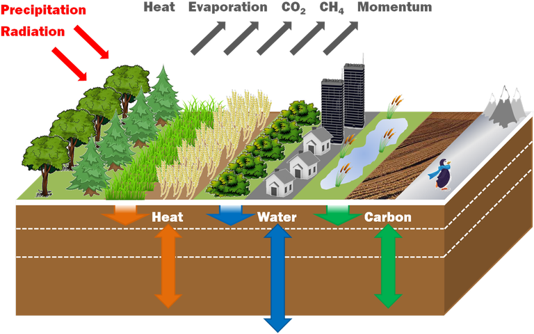
JULES model description diagram

JULES has a tiled model of sub-grid heterogeneity with separate surface temperatures, short-wave and long-wave radiative fluxes, sensible and latent heat fluxes, ground heat fluxes, canopy moisture contents, snow masses and snow melt rates computed for each surface type in a grid-box.

Nine surface types are normally used:

  • Five Plant Functional Types (PFTs): Broadleaf trees, Needleleaf trees, C3 (temperate) grass, C4 (tropical) grass, Shrubs
  • Four non-vegetation types: Urban, Inland water, Bare soil, Land-ice

Except for those classified as land-ice, a land grid-box can be made up from any mixture of the other surface types. Fractions of surface types within each land-surface grid-box are read from an ancillary file or modelled by TRIFFID.

Air temperature, humidity and wind-speed above the surface and soil temperatures and moisture contents below the surface are treated as homogeneous across a grid-box.


Energy balance

Surface energy balance

Surface temperature is interpreted as a surface skin temperature unless the Canopy Heat Capcity model is selected, in which case it is a canopy layer temperature for vegetated tiles. The surface energy balance for each tile includes fluxes of sensible heat and moisture, and latent heat of vaporization for snow-free tiles or sublimation for snow-covered or ice tiles. The heat flux into the ground, combining radiative fluxes below vegetation canopies and conductive fluxes for the unvegetated fraction, is parameterised as a function of the thickness and temperature of the surface soil layer. Radiative canopy fraction is calculated separately if the Canopy Heat Capacity model is selected but is set to zero otherwise. The thermal conductivity is equal to the soil conductivity for snow-free tiles, but is adjusted for insulation by snow.

Resistances and conductances

An aerodynamic resistance for sensible and latent heat fluxes between the surface and the atmosphere over each tile is calculated as a function of the temperature, specific humidity, and windspeed. An addition to the surface resistance factor is defined for evaporation to represent the resistance from the saturated humidity value at the surface temperature within the surface (within the leaf or soil matrix), to the surface humidity. For transpiration, this surface resistance is the reciprocal of the canopy conductance, which depends on the photosynthesis.

Canopy heat capacity

A canopy heat capacity and radiative coupling between the canopy and underlying ground can be used. It depends on the masses of carbon in leaves and stems per unit area of canopy. The areal canopy heat capacity is calculated assuming different specific heat capacities of leaves and wood, based on values given by Jones (1983) and Moore and Fisch (1986).

Evaporation

Surface evaporation is drawn from soil, canopy and snow moisture stores. Evaporation from saturated parts of the surface (lakes, wet vegetation canopies and snow) is calculated at the potential rate (i.e. subject to an aerodynamic resistance only). Evaporation from transpiring vegetation is controlled by the canopy conductance. The ability of vegetation to access moisture at each level in the soil is determined by root density, assumed to follow an exponential distribution with depth.

The evaporative flux extracted from each soil layer is dependent on the soil moisture availability factor. Bare-soil evaporation is extracted from the surface soil layer for both bare-soil tiles and fraction of vegetated tiles. A fraction of the tile is assumed to be saturated and hence has aerodynamic resistance only. This factor is 1 for lake, ice or snow-covered tiles, and varies for a vegetated tile with canopy moisture content and canopy capacity. The urban tile is also given a small surface capacity.

References

Jones, H. G., 1983: Plants and microclimate. A quantitative approach to environmental plant physiology. Cambridge University Press.

Moore, C. J., and G. Fisch, 1986: Estimating heat storage in Amazonian tropical forest. Agric. and Forest Meteorol., 38, 147-168.


Radiation

Surface albedos are specified either as single values for all bands with diagnosed snow albedos or spectral values with prognostic snow albedos.

All-band albedos

Bare soil albedos vary geographically with soil colour. Snow aging is represented by reducing the snow albedo when surface temperature exceeds –2°C

Spectral albedos

The Sellers (1985) two-stream canopy radiation model is used for vegetation albedos in the optional spectral albedo scheme. Separate direct-beam and diffuse albedos in visible and near-infrared wave bands are calculated for each vegetation type.

Snow albedos are calculated using a simplification of the Marshall (1989) parametrization of the Wiscombe and Warren (1980) spectral snow albedo model. The aging of snow is characterized by introducing a prognostic grain size, set to a minimum value for fresh snow and limited to a maximum value.

References

Marshall, S. E., 1989: A physical parametrization of snow albedo for use in climate models. NCAR Cooperative Thesis 123, National Center for Atmospheric Research, Boulder, Co.

Sellers, P. J., 1985: Canopy reflectance, photosynthesis and transpiration. Int. J. Remote Sens., 6(8), 1335-1372

Wiscombe, W. J., and S. G. Warren, 1980: A model for the spectral albedo of snow. I. Pure snow. J. Atmos. Sci., 37, 2712-2733. 24


Hydrology

The partitioning of precipitation into interception, throughfall, runoff and infiltration is described Gregory and Smith (1990) and is applied separately on each tile. Essentially, the rainfall rate is assumed to be distributed exponentially across the area. In addition, if the rainfall is convective, then it is assumed to cover only 30% of the area. This part of the JULES model aims to overcome the problem of GCM-drizzle, whereby every time it rains, a small amount of water covers the entire area, is held on the leaves of the vegetation and re-evaporates, without entering the soil matrix. In practice the rainfall can be intense over small areas and this means the rainfall falls through the vegetation canopy and into the ground. It is possible to turn this feature off if observed rainfall is being used to drive the model (where the rainfall is less frequent but more intense).

References

Gregory, D., and R. N. B. Smith, 1990: Canopy, surface and soil hydrology. Unified Model documentation paper 25, Meteorological Offce, London Rd, Bracknell, Berkshire, RG12 2SY.


Soils

Soil thermodynamics

Subsurface temperatures are updated using a discretised form of the heat diffusion equation, which is coupled to the soil hydrology module. It includes soil water phase changes and the associated latent heat and soil thermal characteristics, which are dependent on soil moisture content (liquid water and ice).

The temperature of the nth soil layer is incremented by the diffusive heat fluxes into and out of the layer, and the net heat flux advected from the layer by the moisture flux. The local soil thermal conductivity (Cox et al, 1999) is modified in the presence of lying snow. The relationship between unfrozen water concentration and temperature can be derived by minimizing the Gibbs free energy.

Soil hydrology

The soil hydrology component of JULES is based on a finite difference approximation to the Richards' equation (Richards, 1931), with the same vertical discretisation as the soil thermodynamics module. The total soil moisture content within a soil layer is incremented by the diffusive water flux flowing in from the layer above, the diffusive flux flowing out to the layer below, the evaporation extracted directly from the layer by plant roots and soil evaporation which is calculated from the total evaporation, based on the profiles of soil moisture and root density. The water fluxes are given by the Darcy equation which depends on the hydraulic conductivity and is the soil water suction. To close the model it is necessary to assume forms for the hydraulic conductivity and the soil water suction as a function of the soil moisture concentration. Either of the dependencies suggested by Brooks & Corey (1964) and van Genuchten et al (1991) can be used in JULES.

Soil carbon

Soil carbon storage is reduced by microbial soil respiration, which occurs at a rate dependent on soil moisture, temperature and soil carbon content, and increased by the total litterfall. The total litterfall is made-up of the area-weighted sum of the local litterfall from each PFT, along with terms due to the large-scale disturbance rate and PFT competition.

The competition is derived by imposing carbon conservation on the soil-vegetation system implying that the NPP of each PFT will be lost entirely as litter once the PFT occupies all of the space available to it.

The moisture dependence of the soil respiration is based on the model of McGuire et al (1992) in which the respiration rate increases with soil moisture content until an optimum value of moisture is reached. Thereafter the rate of respiration is reduced with further increases in soil moisture. The curves presented by McGuire et al (1992) have been approximated by piecewise linear functions in order to minimise the number of additional soil variables required.

References

Brooks RH & Corey AT (1964). Hydraulic properties of porous media. Colorado State University Hydrology Papers 3.

Cox, P. M., R. A. Betts, C. B. Bunton, R. L. H. Essery, P. R. Rowntree, and J. Smith, 1999: The impact of new land surface physics on the GCM simulation of climate and climate sensitivity. Clim. Dyn., 15, 183-203

McGuire, A., J. Melillo, L. Joyce, D. Kicklighter, A. Grace, B.M. Ill and C. Vorosmarty, 1992. Interactions between carbon and nitrogen dynamics in estimating net primary productivity for potential vegetation in North America. Global Biogeochemical Cycles. 6 101-124.

Richards, L., 1931: Capilliary conduction of liquids through porous mediums. Physics, 1, 318-333.

van Genuchten, M., F. Leij, and S. Yates, 1991: The RETC code for quantifying the hydraulic functions of unsaturated soils. Technical Report EPA/600/2-91/065, U.S. Environmental Protection Agency.


Vegetation

Photosynthesis

Stomatal openings are the pathways through which both water and carbon dioxide are exchanged between vegetation and the atmosphere. Consequently, net leaf photosynthesis and stomatal conductance to water vapour are linked. The fluxes of carbon and water vapour are proportional to the gradient of water vapour and carbon dioxide respectively.

Leaf photosynthesis is dependent on a number of environmental variables as well as the internal CO2 concentration. The closure suggested by Jacobs (1994) is used in JULES (Cox et al. 1998, Cox et al. 1999). The leaf photosynthesis models are based on the work of Collatz et al. (1991) and Collatz et al. (1992) for C3 and C4 plants respectively. However, an additional direct soil moisture dependence is introduced as suggested by Cox et al. (1998).

Scaling up

The approach of Sellers et al. (1992) is used for scaling up from the stomatal conductance to the canopy conductance, in which the primary determinants of photosynthesis, mean incident photosynthetically active radiation (PAR) and the maximum rate of carboxylation of Rubisco are assumed to be proportional throughout the plant canopy. The photosynthesis limiting factors are assumed to be the same at every depth in the canopy. As a consequence it is straightforward to integrate the leaf conductance and photosynthesis over the canopy leaf area index to yield canopy conductance and net canopy photosynthesis. The net leaf photosynthesis is calculated by subtracting the rate of dark respiration from the gross photosynthetic rate.

An alternative scaling up procedure is available in JULES. In this case the leaf-to-canopy scaling makes explicit calculations at different levels in the canopy, with the emphasis on a more sophisticated representation of light-interception. Light interception is simulated using the two stream approximation approach of Sellers (1985) which describes absorption and scattering losses of incident radiation for both direct and diffuse radiation separately in the visible and near infrared wavebands. The two stream approach provides a set of equations for variation of direct and diffuse, upward and downward beams through the canopy, calculating PAR as a function of L. The calculated values of PAR(L) also depend on solar zenith angle, direct and diffuse radiation incident at the top of the canopy, leaf angle distribution and leaf radiation properties for each waveband. Using the calculated absorbed light at each layer of the canopy, leaf photosynthesis, leaf respiration and stomatal conductance are calculated at each layer and summed to provide a canopy level value. Based on this additive calculation through the canopy, a canopy level stomatal conductance is defined to allow calculation of overall surface energy partitioning (Jogireddy et al. 2006).

Plant respiration

Plant respiration is split into maintenance and growth respiration. Growth respiration is assumed to be a fixed fraction of the net primary productivity. Leaf maintenance respiration is equivalent to the moisture-modified canopy dark respiration while root and stem respiration is assumed to be independent of soil moisture, but to have the same dependences on nitrogen content and temperature. Thus total maintenance respiration is dependent on the mean leaf nitrogen concentration.

The nitrogen concentrations of root and stem are assumed to be fixed (functional type dependent) multiples of the mean leaf nitrogen concentration. The respiring stemwood is calculated using the “pipemodel" approach in which live stemwood is proportional to leaf area and canopy height (the constant of proportionality is approximated from Friend et al. 1993).

Vegetation dynamics

The dynamic global vegetation model, TRIFFID (Top-down Representation of Interactive Foliage and Flora Including Dynamics), updates the plant distribution depending on the CO2 fluxes at the land-atmosphere interface. The surface CO2 fluxes associated with photosynthesis and plant respiration are calculated at every model timestep (normally 30 minutes), for each of 5 plant functional types while the area covered by a plant type is updated every 10 days. The area covered by each plant type is based on the net carbon available to it and on the competition with other plant types, which is modelled using a Lotka-Volterra approach to intraspecies and interspecies competition (see for example Silvertown, 1987). Competition between natural PFTs is based on a tree-shrub-grass dominance hierachy, with dominant types limiting the expansion of subdominant types. However, the tree types (broadleaf and needleleaf) and grass types (C3 and C4) co-compete with competition coefficients dependent on their relative heights. Some allowance is made for agricultural regions, from which the woody PFTs are excluded, and C3 and C4 grasses are reinterpreted as “crops".

Vegetation carbon content and Leaf Area Index (LAI)

JULES includes parameters describing the maximum and minimum leaf area index values for the given plant functional type, and a “balanced" LAI can be derived (= LAI that would be reached if the plant were in full leaf). The actual LAI depends on the balanced LAI and the phenological status of the vegetation type, which is updated as a function of temperature.

Changes in vegetation carbon density are related allometrically to changes in the balanced LAI. First, it is broken down into leaf, root, and total stem carbon. Then each of these components are related to the balanced LAI. Root carbon is set equal to leaf carbon, which is itself linear in LAI, and total stem carbon is related to the balanced LAI by a power law (Enquist et al. 1998). The local litterfall rate consists of contributions from leaf, root and stem carbon. The leaf turnover rate is calculated to be consistent with the leaf phenology model.

The root turnover rate is set equal to the minimum leaf turnover rate for all PFTs, but the total stem turnover is PFT-dependent to react to the different fractions of woody biomass. There is an additional litter contribution arising from large-scale disturbance which results in loss of vegetated area at the prescribed rate.

Leaf phenology

Leaf mortality rates for the tree-types are assumed to be a function of temperature, increasing as the leaf temperature drops below a threshold value. The leaf turnover rate increases by a factor of 10 when the temperature drops 1°C below the threshold value. The phenological status is updated on a daily basis assuming leaves are dropped at a constant absolute rate when the daily mean value of leaf turnover exceeds twice its minimum value. Budburst occurs at the same rate when leaf mortality drops back below this threshold, and “full leaf" is approached asymptotically thereafter.

This process amounts to a “chilling-days" parameterisation of leaf phenology. A similar approach may be taken for drought-deciduous phenology and for the cold-deciduous phenology of the other (non-tree) PFTs, but neither is included in the current version of JULES.

References

Collatz, G. J., J. T. Ball, C. Grivet, and J. A. Berry, 1991: Physiological and environmental regulation of stomatal conductance, photosynthesis and transpiration: A model that includes a laminar boundary layer. Agric. and Forest Meteorol., 54, 107-136

Collatz, G. J., M. Ribas-Carbo, and J. A. Berry, 1992: A coupled photosynthesis- stomatal conductance model for leaves of C4 plants. Aus. J. Plant Physiol., 19, 519-538

Cox, P. M., C. Huntingford, and R. J. Harding, 1998: A canopy conductance and photo-synthesis model for use in a GCM land surface scheme. J. Hydrology, 212- 213, 79-94

Cox, P. M., R. A. Betts, C. B. Bunton, R. L. H. Essery, P. R. Rowntree, and J. Smith, 1999: The impact of new land surface physics on the GCM simulation of climate and climate sensitivity. Clim. Dyn., 15, 183-203

Enquist, B., J. Brown, and G. West, 1998: Allometric scaling of plant energetics and population density. Nature, 395, 163-166

Friend, A. D., H. H. Shugart, and S. W. Running, 1993: A physiology-based model of forest dynamics. Ecology, 74, 797-797

Jacobs, C., 1994: Direct impact of atmospheric CO2 enrichment on regional transpiration. PhD thesis, Wageningen Agricultural University

Jogireddy VR, Cox PM, Huntingford C, Harding RJ & Mercado L (2006). An improved description of canopy light interception for use in a GCM land-surface scheme: calibration and testing against carbon fluxes at a coniferous forest. Hadley Centre Technical Note 63.

Sellers, P. J., 1985: Canopy reflectance, photosynthesis and transpiration. Int. J. Remote Sens., 6(8), 1335-1372

Silvertown, J., 1987: Introduction to Plant Population Ecology. Longman Scientific and Technical, second edition